Model Interpretability with SHAP
In applied machine learning, there is usually a trade-off between model accuracy and interpretability. Some models like linear regression or decision trees are considered interpretable whereas others, such as tree ensembles or neural networks, are used as black-box algorithms. While this is partly true, there have been great advances in the model interpretability front in the past few months. In this post I will explain one I the newest methods in the field, the so-called SHAP, and show some practical examples of how this method helps interpret the complex GBM model I’m using for making F1 predictions.
But why do we bother with interpreting ML model outputs in the first place? Well, for F1 results it is mostly curiosity I guess, but there’s more than human curiosity. Understanding the most important features of a model gives us insights into its inner workings and gives directions for improving its performance and removing bias. Therefore we can debug and audit the model. The most important reason, however, for providing explanations along with the predictions is that explainable ML models are necessary to gain end user trust (think of medical applications as an example).
What SHAP is
SHAP – SHapley Additive exPlanations – explains the output of any machine learning model using Shapley values. Shapley values have been introduced in game theory since 1953 but only recently they have been used in the feature importance context. SHAP belongs to the family of “additive feature attribution methods”. This means that SHAP assigns a value to each feature for each prediction (i.e. feature attribution); the higher the value, the larger the feature’s attribution to the specific prediction. It also means that the sum of these values should be close to the original model prediction.
SHAP has actually unified six existing feature attribution methods (including the LIME method) and it theoretically guarantees that SHAP is the only additive feature attribution method with three desirable properties:
-
Local accuracy: The explanations are truthfully explaining the ML model
-
Missingness: Missing features have no attributed impact to the model predictions
-
Consistency: Consistency with human intuition (more technically, consistency states that if a model changes so that some input’s contribution increases or stays the same regardless of the other inputs, that input’s attribution should not decrease)
How SHAP is calculated
The calculation of these values is simple but computationally expensive. As stated in the original SHAP paper, the idea is that you retrain the model on all feature subsets S ⊆ F, where F is the set of all features. Shapley values assign an importance value to each feature that represents the effect on the model prediction of including that feature. To compute this effect, a model is trained with that feature present, and another model is trained with the feature withheld. Then, predictions from the two models are compared on the current input i.e. their difference is computed. Since the effect of withholding a feature depends on other features in the model, the preceding differences are computed for all possible subsets of features. The Shapley values are a weighted average of all possible differences and are used as feature attributions.
The authors of SHAP have devised a way of estimating the Shapley values efficiently in a model-agnostic way. In addition, they have come up with an algorithm that is really efficient but works only on tree-based models. They have integrated the latter into the XGBoost and LightGBM packages.
F1-predictor model
Before presenting some examples of SHAP, I will quickly describe the logic behind the model used for making the F1 predictions. So, for each driver I’m calculating some features like the ones mentioned in the feature engineering post. During modelling, for each driver pair I’m calculating the difference between these features and use as label ‘1’ if driver #1 finished ahead of driver #2 and ‘0’ otherwise. The algorithm used by F1-predictor is a LightGBM model which is generally not considered as being interpretable. Therefore, the ranking task is transformed into many binary classification tasks. In a later blog post, I’ll share more details on the model and how these binary predictions are combined to produce the final ranking. The main point here is that all examples below refer to binary classification predictions between driver pairs and the features used are the differences in the respective features of the drivers.
Explaining F1 predictions with SHAP
In general, there is a distinction in the scope of model interpretability. Global interpretability helps understand the relationship between each feature and the predicted values for our entire observation set. It gives us a sense of the magnitude and direction of the impact of each feature on the predicted value.
In contrast, local interpretability describes the impact of each feature on the predicted value for a specific observation. While both are useful, I think it’s usually more important to visualize the impact of features at the local level. Let’s see some examples for both cases. All data below refer to the predictions for the 2017 Abu Dhabi Grand Prix. All plots below have been generated using the SHAP python package.
Global interpretability
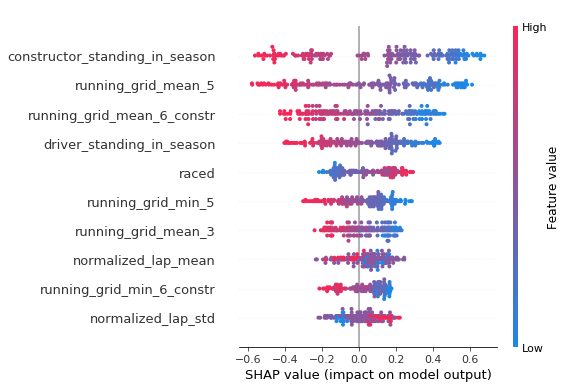
To get an overview of which features are most important for a model we can plot the SHAP values of every feature for every sample. The plot below sorts features by the sum of SHAP value magnitudes over all samples, and uses SHAP values to show the distribution of the impacts each feature has on the model output. The color represents the feature value (red high, blue low). This plot refers to the top-10 features used to predict the race results:

The plot reveals that low values of the ‘grid’ (i.e. starting position) feature lead to driver #1 finishing ahead of driver #2. As a reminder, the ‘grid’ feature here is the difference in starting position between the drivers. That is, if driver #1 starts in P1 and driver #2 at P7, then the grid feature is 1 – 7 = -6. Therefore, we confirm our intuition that the starting position in the most important predictor of the final race result and the model has learned this relationship. We can also see that the time difference in Q1 times is, somewhat strangely, slightly more important that Q2 and Q3 time differences. This could be because all drivers participate in Q1 while only few of them go through to Q2 and Q3. Lastly, the constructor standing has a significant impact since the car is as, or even more, important than the driver nowadays.
Now, let’s see the same plot for the model predicting qualifying results:
This reveals how important the car is, especially during qualifying. It is actually the most important predictor of qualifying performance. The 2nd feature is the average, over the past 5 races, of each driver’s performance in qualifying while the 3rd one is the average over the past 3 races (the ‘6’ in the plot comes from the fact that there are two drivers for each team) of the constructor’s performance in qualifying.
So far, so good. Everything seems inline with what we’d expect based on our experience from F1 races. Now, let’s dive into the SHAP values for individual predictions.
Local interpretability
Here’s the first example. The model gave only a 2% chance of Alonso finishing ahead of Hamilton in the race. Let’s see why the models thinks so. The features in blue push the predictions towards 0% while the opposite holds true for the features in red.
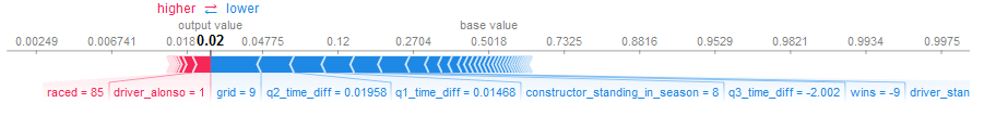
As expected, the fact that Alonso starts 9 positions below Hamilton is the most important factor. Their difference n Q1 and Q2 also helps as does the fact that Mercedes is way ahead of McLaren in the constructors championship. The main reason that the probability is 2% instead of something lower is the fact that Hamilton is against Alonso, maybe the greatest F1 driver ever, who has also raced 85 more races compared to Hamilton.
Below is another comparison, between teammates this time; Vettel and Raikonnen. The former was given an 83% probability of finishing ahead of the latter:
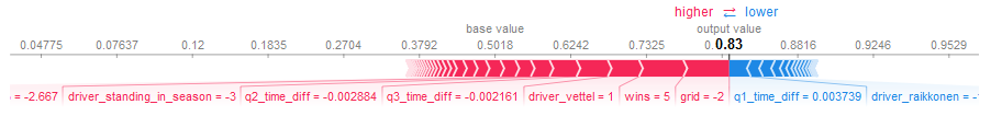
Again, the reasons behind the predictions make an intuitive sense. Vettel is predicted to come ahead of Raikonnen due to their difference in their starting position, due to the fact that Vettel has more wins than Raikonnen and due to the differences in Q2 and Q3 qualifying times. However, the fact that Raikonnen was faster in Q1, gives him some chances as well.
Let’s also see an example for qualifying. The plot below shows why Bottas had a 74% chance of qualifying ahead of Max Verstappen:

Since Bottas drives for Mercedes, arguably the best car out there, it’s normal that this has affected the predictions. In addition, Bottas had stronger qualifying performances in the past 5 races (shown as ‘running_grid_mean_5’ here). On the other hand, the fact that Max is driving for Red Bull increases his chances of qualifying ahead of Bottas.
Conclusion
I think that the examples contradict the notion that you have to either select an explainable model or a more complex – and therefore more accurate – one. The explanations given using an accurate and complex Gradient Boosting Machine model were as clear as a linear model could get and made total intuitive sense. This also highlights the strengths of SHAP in providing accurate and consistent explanations.
There is much more in model interpretability, however I hope this post gives a head start on those wondering if and how they can approach such a task. There are great resources out there on this topic and I’m listing some of them I found interesting below.
Resources on ML model interpretability:
16 thoughts on “Model Interpretability with SHAP”
What software or library did you use to make the plots? Particularly the last ones!
All plots were made with this python library.
Hi,
When will you publish the predictions for Bahrain :)?
Just published them: https://www.f1-predictor.com/bahrain-gp-2018/ 🙂
Hi Stergios,
How do you make your plot return the probability? Mine returns log odds.
Regards
Germayne
You should add the correct ‘link’ like so:
shap.force_plot(shap_values[0,:], X.iloc[0,:], link=shap.LogitLink())thank you stergios! i found the solution as well
https://github.com/slundberg/shap/issues/75
Hi Stergios,
How can I install this in my env in lunux. I tried ‘pip install shap’ but got kicked out with a ‘gcc’ failed error.
Thanks
Hi Deepak,
I don’t know why you got this error. The installation was straightforward for me (on Windows thought).
You can raise an issue on github.
Raised an issue on Github. Thanks!
Can SHAP be used to explain the results of *any* classifier?
Theoretically yes. I think the existing implementation works with scikit, Xgboost and LightGBM models.
What do the base value and the output value represent?
Example: for a classification problem such as this ( https://slundberg.github.io/shap/notebooks/Iris%20classification%20with%20scikit-learn.html)
where the classifier is categorizing into class 0, 1 or 2 – what is the notion of base value and output value?
If it were possible, Please do share the code for the above analysis.
Hi Akhil,
I’ve never used SHAP for multiclass classification. I guess the base value is the average prediction probability for that class and the output value is the prediction for the given sample.
As for my analysis, I will share the code when I find some time to clean it up.
did you get an answer ? i am using it with multiclass and did not understand the meaning of the base value and output value?
Rabab please ask the question on Github. Get back to us if you find out. I’m interested to learn that.